Understanding and Implementing Automatic Differentiation
\[ \DeclareMathOperator{\expt}{expt} \DeclareMathOperator{\mul}{mul} \DeclareMathOperator{\add}{add} \DeclareMathOperator{\derivative}{derivative} \]
Automatic differentiation is a technique that allows programs to compute the derivatives of functions. It is vital for deep learning and useful for optimization in general. For me, it’s always been dark magic, but I recently thought of a nice way to implement it and made a little library. This blog post takes you along the journey of discovering that implementation. Specifically, we will be implementing forward mode automatic differentiation for scalar numbers.
This post requires some knowledge of differential calculus. You’ll need to know basic derivative rules, the chain rule, and it’d help to know partial derivatives. If you’ve taken an introductory calculus course, you should be fine.
The code is in Racket. If you don’t know Racket, you should still be able to follow along. I’ll explain the Racket-y stuff. Don’t let the parentheses scare you away!
|
|
1 Introduction
Gradient descent is an optimization technique that involves derivatives. You have some quantity you want to optimize, let’s say \(y\), and you have some variable \(x\) that you can adjust that affects \(y\). What value of \(x\) maximizes \(y\)? Using gradient descent, if we take the derivative of \(y\) with respect to \(x\), \(\frac{dy}{dx}\), that tells us how changing \(x\) affects \(y\). If the derivative is positive, increasing \(x\) increases \(y\). If it is negative, increasing \(x\) decreases \(y\). If it is positive and large, increasing \(x\) increases \(y\) a lot. So, if we’re trying to maximize \(y\), we’d change \(x\) in the same direction as the derivative. If it’s positive, we increase \(x\) to make \(y\) greater. If it’s negative, we decrease \(x\) to make \(y\) greater. This will end up maximizing \(y\) (at least, reaching a local maximum). This is a very useful technique and it is fundamental to deep learning with neural networks. Awesome! But how do you compute the derivative of a function with respect to its input?
Naively, you might try something like this:
| |||
| > (define (square x) (* x x)) | |||
| > (derivative square 5 0.01) | |||
|
10.009999999999764 |
For those not familiar with Racket, it has prefix arithmetic. This means that instead of writing \(a + b\), we write (+ a b). It also has a lot of parentheses, which can be tricky to read. You can mostly ignore them and just read based on indentation.
Here, we define a function called derivative which takes in 3 arguments: a Number -> Number function f, a number x representing the input, and a number h representing the step size of the derivative. The body of derivative has a lot of parentheses and prefix arithmetic that is hard to read. Here is what this looks like in normal math notation:
\[\derivative(f,x,h) = \frac{f(x+h) - f(x)}{h}\]
This is reminiscent of the limit definition of a derivative that you learn about in an introductory calculus course.
\[\frac{df}{dx} = \lim_{h \to 0} \frac{f(x + h) - f(x)}{h}\]
This can work well enough as an approximation, but you need a small h and there will always be rounding error, as we saw in the square example. Another issue is that if we have a multi-argument function, we’d have to run the function many times to get the partial derivatives. This is not ideal. What we’d like is to be able to run the function once, inspect several derivatives after, and get exact derivatives. This is the goal of automatic differentiation.
Here is a sneak peek of what we will implement:
| > (require number-diff) |
| > (define (f a b) (*o a b)) |
| > (define a (number->dnumber 5)) |
| > (define b (number->dnumber 3)) |
| > (define y (f a b)) |
| > (dnumber->number y) |
|
15 |
| > (dnumber->number (derivative y a)) |
|
3 |
| > (dnumber->number (derivative y b)) |
|
5 |
*o is just my version of multiplication that supports derivatives.
We’ll even get higher order derivatives!
| > (dnumber->number a) |
|
5 |
| > (define y (*o a a)) |
| > (dnumber->number y) |
|
25 |
| > (dnumber->number (derivative y a)) |
|
10 |
| > (dnumber->number (derivative (derivative y a) a)) |
|
2 |
| > (dnumber->number (derivative y a #:order 2)) |
|
2 |
2 How?
2.1 The Math
I first encountered automatic differentiation when I was learning about neural networks in college. In the popular neural networks libraries, you define your neural network, and this constructs a computation graph. A computation graph stores the operations, inputs, and outputs of a computation. Here is an example from PyTorch documentation:
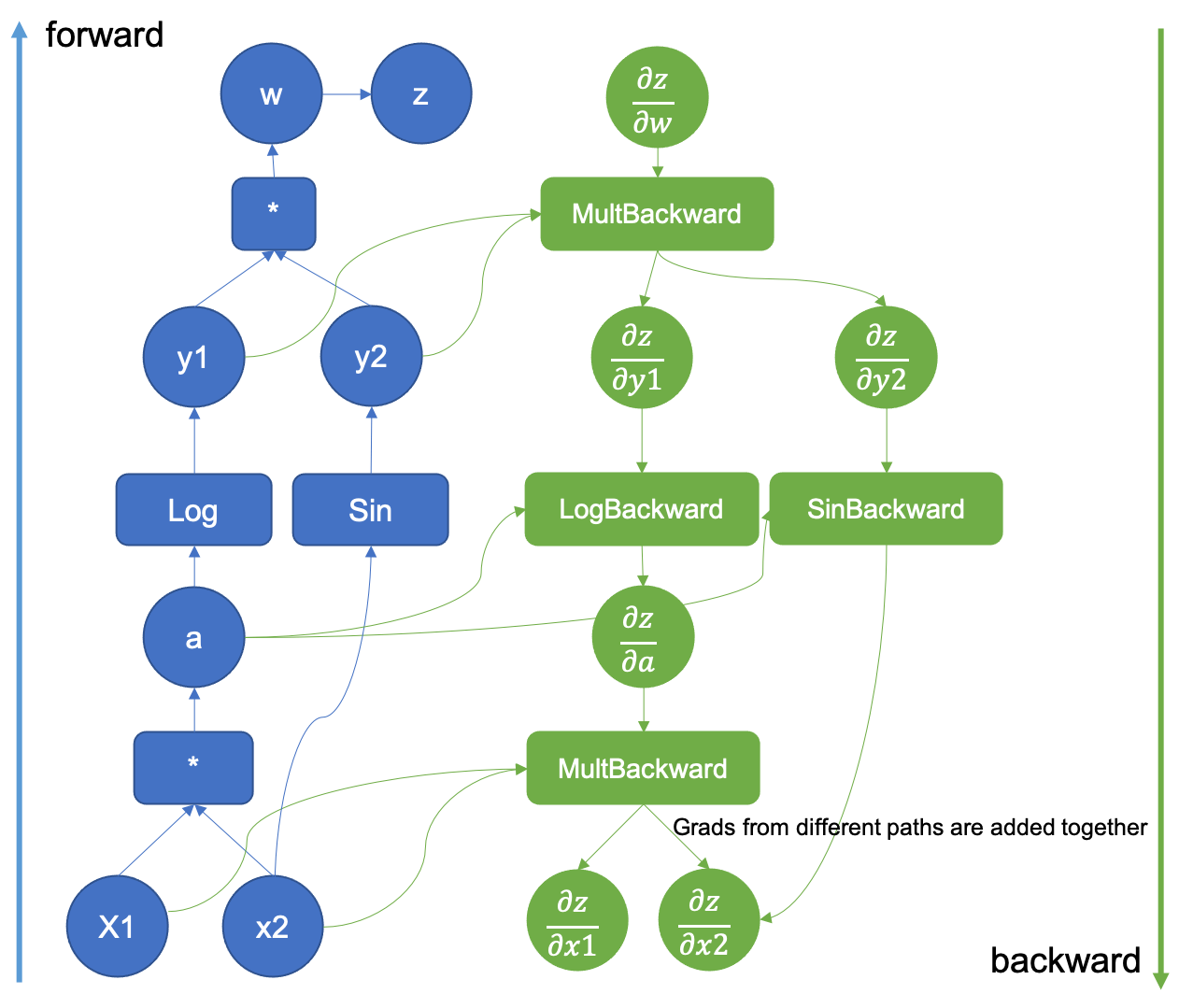
This represents the computation \(\log (x_1 x_2) \sin (x_2)\). Intermediate results like \(x_1 x_2\) get their own nodes (\(a\)).
The green part of the image shows how the derivatives are calculated. Each operator, like multiplication, logarithm, etc., knows how to compute the derivatives of its result with respect to its inputs. The rest is just applying the chain rule and adding up partial derivatives as appropriate.
There is a lot going on here, so don’t worry about fully understanding this picture yet. We will get there. The key idea is that a computation can be expressed as a graph, where inputs are like leaves, and operations are like nodes. And each node is a tiny computation which is easy to compute the derivatives for.
Let’s start by thinking about some core operators and their derivatives:
\[ \mul(a,b) = ab \]
What are the derivatives?
\[ \frac{\partial \mul}{\partial a} = b \]
\[ \frac{\partial \mul}{\partial b} = a \]
This comes from the rule for multiplying a constant:
\[ \frac{d}{dx} cx = c \]
Remember, taking the partial derivative means treating the other arguments as constants.
Ok, what about addition?
\[ \add(a,b) = a + b \]
\[ \frac{\partial \add}{\partial a} = 1 \]
The derivative is 1 because \(\frac{da}{da} = 1\) and \(\frac{da}{db} = 0\). Using the sum rule, we get \(1+0=1\).
\[ \frac{\partial \add}{\partial b} = 1 \]
This is 1 for the same reason.
What about Exponentiation?
\[ \expt(a,b) = a^b \]
\[ \frac{\partial \expt}{\partial a} = ba^{b-1} \]
This derivative treats \(b\) as a constant, which makes this the derivative of a polynomial. So we use the power rule.
\[ \frac{\partial \expt}{\partial b} = a^b \ln(a) \]
This derivative treats \(a\) as a constant, which makes this the derivative of an exponential. So we use the exponential rule.
What if things get more complicated? How would you compute this derivative?
\[ y = (3x + 1)^2 \]
\[ \frac{dy}{dx} = ? \]
You use the chain rule!
\[ \frac{dy}{dx} = \frac{dy}{du} \frac{du}{dx} \]
Let \(u_1 = 3x+1\).
\[y = u_1^2\]
Now we can use the power rule:
\[ \frac{dy}{du_1} = 2u_1 \]
We can easily tell that \(\frac{du_1}{dx} = 3\), but let’s do this mechanically to get an idea of how we might automate it:
Let \(u_2 = 3x\)
\[u_1 = u_2 + 1\]
Now we can use the derivative of \(\add\):
\[ \frac{du_1}{du_2} = 1 \]
Finally, we use the constant factor rule:
\[\frac{du_2}{dx} = 3\]
Now, we can go back up the chain:
\[\frac{du_1}{dx} = \frac{du_1}{du_2}\frac{du_2}{dx} = 1 \cdot 3 = 3\]
\[\frac{dy}{dx} = \frac{dy}{du_1}\frac{du_1}{dx} = 2u_1 \cdot 3 = 6u_1 = 6(3x+1)\]
We did it!
Now we can almost see a recursive algorithm for computing derivatives. If a computation is just a bunch of nested simple operations like addition and multiplication, we can compute the derivative by applying the chain rule and using the partial derivatives of our operators at each step. There’s just one tricky bit: What if \(x\) shows up twice?
In other words, if we have \(f(a,b)\) and we know \(\frac{\partial f}{\partial a}\) and \(\frac{\partial f}{\partial b}\), how do we compute \(\frac{df(x,x)}{dx}\)?
One way of thinking about a derivative is asking "if we adjust this input a little bit, how does the output change?". So if \(x\) shows up in multiple places, we are making several inputs change the same way and seeing how the output is affected. If we know how each input changes the output, we just add up all of those little changes to get the big, total change. Concretely, this means we just add the partial derivatives together.
Here is an example:
\[\frac{d \add(x,x)}{dx} = 1 + 1 = 2\]
The partial derivative of \(\add\) with respect to each input is 1. So we get \(1+1=2\). This makes sense because \(x+x=2x\) and \(\frac{d2x}{dx} = 2\).
One more example:
\[\frac{d \mul(x,x)}{dx} = x + x = 2x\]
The partial derivative of \(\mul\) with respect to each input is the other input. So we get \(x + x = 2x\). This makes sense because \(x \cdot x = x^2\) and \(\frac{dx^2}{dx} = 2x\).
In general, for computing \(\frac{\partial f(a,b)}{\partial x}\), \(a\) and \(b\) might be \(x\), might depend on \(x\), or might not depend on \(x\) at all. To account for this, we use the chain rule and this "partial derivative sum rule" (the technical term for this is the total derivative):
\[\frac{d f(a,b)}{d x} = \frac{\partial f(a,b)}{\partial a}\frac{d a}{d x} + \frac{\partial f(a,b)}{\partial b}\frac{d b}{d x}\]
If \(a = x\), \(\frac{d a}{d x} = 1\). If \(a\) depends on \(x\), \(\frac{d a}{d x}\) be some value. If it does not depend on \(x\), it will be 0.
For example, let’s compute \(\frac{d}{dx} (5x)^2\):
\[\frac{d \expt(5x,2)}{dx} = \frac{d \expt(5x,2)}{d5x}\frac{d5x}{dx} + \frac{d \expt(5x,2)}{d2}\frac{d2}{dx}\] \[\frac{d \expt(5x,2)}{dx} = 2 \cdot 5x \cdot 5 + \frac{d \expt(5x,2)}{d2} \cdot 0\] \[\frac{d \expt(5x,2)}{dx} = 50x\]
Notice that, since 2 does not depend on \(x\), its derivative was 0, and that term did not contribute to the overall derivative.
Normally, you don’t think of something like \((5x)^2\) as a sum of two partial derivatives like this. You don’t bother taking the derivative of the 2. You normally don’t have to worry about it since it just ends up adding 0. But since we’re trying to automate this, we need to be general and account for the possibility that \(x\) might show up in the base and the exponent when differentiating an exponential, or generally, multiple times in any function. In fact, we should’ve done the same thing for \(\frac{d5x}{dx}\) and added up \(\frac{d\mul(5,x)}{dx}\frac{dx}{dx} and \frac{d\mul(5,x)}{d5}\frac{d5}{dx}\) to get \(5 \cdot 1 + x \cdot 0 = 5\).
Side note: You may have been wondering, "where’s the product rule?" In fact, the product rule is not fundamental! It can be derived from the constant factor rule, the chain rule, and this "partial derivative sum rule":
\[\frac{d}{dx}f(x)g(x) = \frac{d}{dx}\mul(f(x),g(x)) = \frac{\partial \mul(f(x),g(x))}{\partial f(x)}\frac{df}{dx} + \frac{\partial \mul(f(x),g(x))}{\partial g(x)}\frac{dg}{dx}\] \[= g\frac{df}{dx} + f\frac{dg}{dx}\]
Nice!
Now, we’re ready for the recursive algorithm to compute (partial) derivatives.
\[\derivative(x,x) = 1\] \[\derivative(c,x) = 0\] where \(c\) is a constant and not \(x\). \[\derivative(f(u_1,u_2, \cdots , u_n), x) = \sum_{i=0}^{n} \frac{\partial f(u_1,u_2, \cdots , u_n)}{\partial u_i} \cdot \derivative(u_i, x)\]
The base cases are the constant rule and the fact that \(\frac{dx}{dx} = 1\). The recursive case is the interesting bit. For each input to the computation, we apply the chain rule, which involves a special partial derivative and a recursive call. And we add up those applications of the chain rule for each input.
Why don’t we need a recursive call for \(\frac{\partial f(u_1,u_2, \cdots , u_n)}{\partial u_i}\)? We don’t need one because \(f(u_1,u_2, \cdots , u_n)\) is some simple operation like \(\mul\) or \(\add\) or \(\expt\) for which we know how to compute the partial derivatives. Since we are differentiating with respect to an immediate input, \(u_i\), this knowledge is all we need and we don’t need to apply the chain rule or make a recursive call.
This is all very hand-wavy, but it’ll become more concrete soon, I promise!
At this point, that computation graph picture from earlier should start to make some sense. In particular, the green part. Each operator knows how to compute the derivatives of its result with respect to its inputs. That’s the "backward" stuff. And it says "Grads from different paths are added together" (grad=gradient=derivative for our purposes) because of that "partial derivative sum rule". In their example, \(x_2\) shows up twice in the computation, so we need to account for that by adding multiple partial derivatives together.
2.2 The Implementation
We have a (somewhat hand-wavy) algorithm for computing derivatives. Now, we have to actually implement it.
2.2.1 A Data Representation
Let’s think about the pieces we’ll need:
We’ll need operators which can compute partial derivatives of their result with respect to their input(s). We’ll also need constants to pass to these operators. It is unclear how "variables" will be represented, so let’s not think about that for now. In order to compute the derivative of a result with respect to some input after the computation is complete, we’ll need to remember what inputs were involved in a computation.
So a computation will need to store the value of its result and its inputs, at a bare minimum. Its inputs may be results of other computations too. This means there will be a tree structure where a computation has a node that stores its result and has children for its inputs. At the leaves of this tree will be constants. We can think of a constant as a computation with no inputs that has itself as a result. Let’s write a data definition for this tree:
| (struct computation [value inputs] #:transparent) |
| ; A Computation is a |
| ; (computation Number (listof Computation)) |
| ; It represents the result of a numerical computation |
| ; Examples: |
| (define const2 (computation 2 (list))) |
| (define const3 (computation 3 (list))) |
| (define prod23 (computation 6 (list const2 const3))) |
In Racket, struct creates a structure type. It’s like a struct in C, or a data class in Python or Java. It only has fields, no methods. #:transparent automatically implements conversion to a string for our structure type so we can print it, and semicolon creates a line comment. The list function creates lists, so (list) creates the empty list.
This is on the right track, but it’s not enough information to compute derivatives. We have no way to compute the derivative of the result with respect to an input. What else do we need in the tree?
Let’s take another look at the recursive case of our algorithm. The recursive step involves computing the partial derivatives of the result with respect to one of its direct inputs, \(\frac{\partial f(u_1,u_2, \cdots , u_n)}{\partial u_i}\). This is the missing piece. We just have to figure out how to represent this information in our tree.
One option would be to do what PyTorch seems to do: Store some information about the operation in a node. In our prod23 example, we’d store something representing multiplication in the tree. In the PyTorch, we see that the computation graph stores something for * and something called MultBackward. MultBackward is something that knows how to compute the derivative of a product with respect to its input factors. With this design, we could store a function in the tree that can be used to compute the derivative of the result with respect to each input. Each operator would be responsible for computing its result and creating a node containing that result, a function for computing derivatives, and the inputs.
Another option is to pre-compute these derivatives and store the value of each derivative in the tree with its corresponding input. With this design, each operator would be responsible for computing its result, computing the derivative of the result with respect to each input, and creating a node containing the result, the inputs, and the derivatives of the result with respect to each input. This is the design I chose for my implementation, and the one we’ll implement together.
Both options have pros and cons. This is just the design I came up with. One good thing about this design is that it generalizes nicely to higher order derivatives, which was a goal of my implementation.
Let’s think about an example to make this more concrete. Let’s say we have some operator f and some inputs a and b. The computation is (f a b) (that’s how we write \(f(a,b)\) in Racket). Let’s call the result y. Keep in mind that a, b, and y are not plain numbers. They are trees. In this case, a and b will be direct children of y since they are inputs to the computation that produced y.

The tree for y will store the numerical value of the result of the computation, and for its children, it will have a and b. It will also store the numerical value of \(\frac{\partial y}{\partial a}\) and the numerical value of \(\frac{\partial y}{\partial b}\).
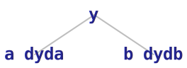
a and b may have children of their own, but we exclude them from these diagrams. dyda and dydb are plain numbers, not trees.
If we’re trying to compute (derivative y x), where x may be some input to the computation that produced a, the first thing we’ll encounter is the node y, which came from (f a b), and we’ll do the recursive step. According to our algorithm, we need to compute
\[\frac{\partial y}{\partial a} \cdot \derivative(a,x) + \frac{\partial y}{\partial b} \cdot \derivative(b,x)\]
Those partial derivatives are what we have in our tree. The rest is just making recursive calls and applying the chain rule. Now we have enough information to compute derivatives! Let’s write a data definition:
| > (struct dnumber [value inputs] #:transparent) |
| ; a DNumber ("differentiable number") is a |
| ; (dnumber Number (listof DChild) ) |
| ; It represents the result of a differentiable computation. |
| ; ‘value‘ is the numerical value of the result of this computation |
| ; ‘inputs‘ associates each input to this computation with the numerical value of its partial derivative |
| > (struct dchild [input derivative] #:transparent) |
| ; A DChild is a |
| ; (dchild DNumber Number) |
| ; It represents an input to a differential computation. |
| ; ‘input‘ is the DNumber that was supplied as an input to the parent computation |
| ; ‘derivative‘ is the numerical value of the partial derivative of the parent result with respect to this input. |
A DNumber stores the value of its result as a plain number and, for each input, the input’s DNumber and the partial derivative of the result with respect to that input as a plain number.
Let’s look at \(2 \cdot 3\) as an example:
| > (define const2 (dnumber 2 (list))) |
| > (define const3 (dnumber 3 (list))) |
| > (define prod23 (dnumber 6 (list (dchild const2 3) (dchild const3 2)))) |
We create dnumbers for the constants 2 and 3. Since these are constants, they have no children ((list) creates an empty list).
We then construct a node for the multiplication which stores the value of the result (6) and each input paired with its derivative.
The result of \(2 \cdot 3\) is 6. The inputs are 2 and 3. Recall the derivatives of the \(\mul\) multiplication operator:
\[\frac{\partial \mul(a,b)}{\partial a} = b\] \[\frac{\partial \mul(a,b)}{\partial b} = a\]
The derivative of the product with respect to one of its factors is the other factor. So the derivative of prod23 with respect to const2 is the plain number 3.
We are pre-computing that \(\frac{\partial f(u_1,u_2, \cdots, u_n)}{\partial u_i}\) from our algorithm and storing it directly in our tree as the derivative field (the second argument of the constructor) of a dchild. Each dchild contains the tree for that input \(u_i\) and the value of \(\frac{\partial f(u_1,u_2, \cdots, u_n)}{\partial u_i}\). This is exactly what we need for the recursive case.
Let’s implement our multiplication operator:
| |||||
| > (mul const2 const3) | |||||
|
(dnumber 6 (list (dchild (dnumber 2 '()) 3) (dchild (dnumber 3 '()) 2))) | |||||
| > prod23 | |||||
|
(dnumber 6 (list (dchild (dnumber 2 '()) 3) (dchild (dnumber 3 '()) 2))) |
In the output, we see '() instead of (list). That’s just another way of writing it.
The function dnumber-value is a field-accessor function that is automatically generated from the struct declaration. This field contains the numerical result of the computation. Since Racket’s * function expects plain numbers, we have to get the numerical values of the inputs with dnumber-value before passing them to *.
We also have to do this when creating the dchildren. This is because the derivative field of a dchild must be a plain number. However, the input field must be a DNumber, so we pass the input itself in as the first argument to the dchild constructor and the numerical value of the other input as the second argument.
Let’s do another example, this time \(4 + 5\):
| > (define const4 (dnumber 4 (list))) |
| > (define const5 (dnumber 5 (list))) |
| > (define sum45 (dnumber 9 (list (dchild const4 1) (dchild const5 1)))) |
Recall the derivatives of the \(\add\) addition operator:
\[\frac{\partial \add(a,b)}{\partial a} = 1\] \[\frac{\partial \add(a,b)}{\partial b} = 1\]
Now let’s implement it:
| |||||
| > (add const4 const5) | |||||
|
(dnumber 9 (list (dchild (dnumber 4 '()) 1) (dchild (dnumber 5 '()) 1))) | |||||
| > sum45 | |||||
|
(dnumber 9 (list (dchild (dnumber 4 '()) 1) (dchild (dnumber 5 '()) 1))) |
Great! Now we have a few differentiable operators. Adding more operators will be just like this. We extract the values from the arguments, compute the result using the inputs’ values and built-in arithmetic operators from Racket, and then create a list of dchildren mapping each input to the value of the derivative of the result with respect to that input.
Now we’re finally ready to start implementing the derivative function!
2.2.2 The Derivative!
Before we actually implement the derivative, there are a few things we have to address.
Here is a problem:
What should (derivative sum44 const4) be? If we apply the "partial derivative sum rule", it should be \(1 + 1 = 2\). This makes sense because \(x + x = 2x\) and \(\frac{d}{dx} 2x = 2\).
Let’s look at another example:
| > (define const-four (dnumber 4 (list))) | ||
|
Should (derivative sum4-four const4) also be 2? const4 and const-four are both constant computations that have the result 4 and no inputs. But should they be treated as the same? What does it mean to be the same?
Let’s take a step back and think about a real example where this matters:
Here, \(f(x) = x + 4\). \(\frac{df}{dx} = 1\). If we consider const4 and any other constant 4 to be the same, the derivative of f with respect to x would be 1 for all inputs except for any constant 4, in which case it is 2. This doesn’t make sense. But const4 is obviously the same as const4, so how can we tell these two 4 constants apart?
Racket has a few different equality functions. The one we want is eq?. By convention, when a function returns a boolean, the name ends in a question mark, pronounced "huh". So eq? is pronounced "eek-huh". Anyway, here’s how it works:
| > (define nums (list 1 2 3)) |
| > (eq? nums nums) |
|
#t |
| > (define numbers (list 1 2 3)) |
| > (eq? nums numbers) |
|
#f |
| > (eq? (list 1 2 3) (list 1 2 3)) |
|
#f |
| > (define nums-alias nums) |
| > (eq? nums nums-alias) |
|
#t |
In racket, #t means true and #f means false.
eq? returns #t when both objects are aliases of each other. If both objects were created from different constructor calls, they will not be eq? to each other. If you know Java, it behaves just like ==. This is often called reference equality or identity equality.
| > (eq? const4 const4) |
|
#t |
| > (eq? const-four const-four) |
|
#t |
| > (eq? const4 const-four) |
|
#f |
| > (eq? (dnumber 4 (list)) (dnumber 4 (list))) |
|
#f |
| > (define const4-alias const4) |
| > (eq? const4-alias const4) |
|
#t |
This is exactly what we want! We consider two dnumbers the same if they are eq? to each other. This is a little confusing, but it’s necessary to distinguish between different computations that coincidentally have the same tree data, but aren’t associated with each other. This is exactly the behavior that we need for variables, like our \(x + 4\) example earlier.
What if const4 shows up twice as an input in a computation like in sum44? In that case, our tree isn’t actually a tree. It’s a directed acyclic graph. DAG for short. This is like a tree, except a node can be a child of multiple nodes. However, there cannot be cycles. In other words, a node cannot be an input to itself, or an indirect input to itself. This is why it’s called a computation graph and not a computation tree.
Now we’re finally ready to implement the derivative function!
| ; (DNumber DNumber -> Number) | ||||||||
| ; Compute the partial derivative of y with respect to x. | ||||||||
|
First, let’s cover some Racket stuff.
(if cond-expr then-expr else-expr) is like an if statement in most languages, except it’s just an expression that evaluates to one of its branch expressions. If cond-expr evaluates to anything other than #f, the result is then-expr. Otherwise, the result is else-expr.
(let ([var val-expr]) body-expr) is a local variable definition expression. It binds var to the result of val-expr and var is in scope in body-expr. The whole expression evaluates to the result of body-expr. You can also bind multiple variables like (let ([x 1] [y 2]) (+ x y)).
for/sum is like a for-loop, but it is an expression and calculates the sum of the results from each iteration.
For example:
| > (define words (list "My" "name" "is" "Mike")) | ||
| ||
|
12 |
Again, dnumber-inputs, dchild-input, and dchild-derivative are field accessor functions. In the inner let, we bind the input DNumber to the variable u and the (partial) derivative of y with respect to u to the variable dydu. Remember, we store this derivative directly in the computation graph.
Now let’s think about what’s going on. If y and x are the same, then the derivative is 1. That’s the first branch of the if.
That’s also the first case of the algorithm:
\[\derivative(x,x) = 1\]
Otherwise, we apply the "partial derivative sum rule" and the chain rule. That’s the recursive case of our algorithm.
\[\derivative(f(u_1,u_2, \cdots , u_n), x) = \sum_{i=0}^{n} \frac{\partial f(u_1,u_2, \cdots , u_n)}{\partial u_i} \cdot \derivative(u_i, x)\]
What about this case?
\[\derivative(c,x) = 0\] where \(c\) is a constant and not \(x\).
It’s actually hidden in the for/sum part. If y is a constant (no inputs) and it is not eq? to x, the for/sum will loop over an empty list of inputs. The sum of nothing is 0, so we return 0.
If x does not show up in y’s computation graph, we’ll never get the eq? case. The only base case we’ll hit is the implicit unequal constant base case, which returns 0. Since each base case returns 0, each recursive call will involve multiplying dydu by 0, which will produce 0. And since we’re just adding those together for each input, we’ll be adding up a bunch of zeros, which will produce 0. By induction, we’ll get 0 for the whole derivative if x does not appear in y.
Let’s test out our implementation:
| > (derivative const4 const4) | ||
|
1 | ||
| > (derivative const4 const3) | ||
|
0 | ||
| > (derivative const4 const-four) | ||
|
0 | ||
| > (derivative sum44 const4) | ||
|
2 | ||
| > (derivative sum44 const-four) | ||
|
0 | ||
| > (derivative (add-4 const3) const3) | ||
|
1 | ||
| > (derivative (add-4 const4) const4) | ||
|
1 | ||
| > (define (double x) (add x x)) | ||
| > (derivative (double const3) const3) | ||
|
2 | ||
| > (derivative (double const3) const4) | ||
|
0 | ||
| > (define (square x) (mul x x)) | ||
| > (derivative (square const4) const4) | ||
|
8 | ||
| > (derivative (square const3) const3) | ||
|
6 | ||
| > (derivative (mul const3 const4) const4) | ||
|
3 | ||
| > (derivative (mul const3 const4) const3) | ||
|
4 | ||
| ||
|
84 |
We did it! Now, if you add some more differentiable operators, you can do all sorts of things. You can do gradient descent, you can do analysis, you can implement neural networks, and anything else involving derivatives.
Let’s implement some more operators:
| ||||
| > (e^x const4) | ||||
|
(dnumber 54.598150033144236 (list (dchild (dnumber 4 '()) 54.598150033144236))) | ||||
| > (derivative (e^x const4) const4) | ||||
|
54.598150033144236 | ||||
| ||||
| ||||
|
sub and div are interesting. They don’t directly construct the resulting DNumber. They just use other operators! If we implement a sufficient core library of mathematical operators, it’s easy to define more complicated differentiable functions in terms of those core functions without having to think about derivatives at all.
Automatic differentiation is useful, but if I’m being honest, the real reason I wrote this blog post was because of how much I love that recursive case. Once I wrote that, I wanted to show everybody. You can see the chain rule so clearly!
Our implementation of derivative shows the essence of automatic differentiation. The derivative of something with respect to itself is 1, and the derivative of some function call with respect to a possibly indirect input is the sum over the chain rule applied to each input. Beautiful!
What about higher order derivatives? To achieve this, can we just apply derivative twice? Unfortunately, no. The signature doesn’t line up. derivative returns a plain number, so we can’t pass that as y to another call to derivative. But what if we returned a DNumber instead? That DNumber would have to represent the computation that produced the derivative itself. Is this even possible?
Yes! But it’s not trivial. Think about how this might work and what problems you would run into with a function like \(\expt(a,b) = a^b\).
This post is already pretty long and a lot to digest, so I wont get into higher order derivatives here. But I will in part 2!